Analyze surface velocities of a video with velocimetry#
This notebook shows how to use a camera configuration, and a video to estimate velocities at the surface. It also demonstrates the important impact of filtering of spurious or noisy velocities on the end result. We go through the following steps:
Read a pre-defined camera configuration from file (we use the one prepared in notebook 1)
Open a video, and provide the predefined camera configuration to it.
Project frames to a planar projection
Estimate surface velocities with Particle Image Velocimetry
Filter raw velocities using several temporal and spatial filters
Plot results in the camera objective
[1]:
import pyorc
import matplotlib.pyplot as plt
import xarray as xr
import cartopy
import cartopy.crs as ccrs
import cartopy.io.img_tiles as cimgt
from dask.diagnostics import ProgressBar
from matplotlib import patches
load our camera configuration#
If you didn’t do notebook 01, first go through that notebook to understand how a camera configuration is made.
Below, the camera configuration is loaded back into memory, and used to open a video file. We only need a couple of seconds video, so we use frame 0 until frame 125 only. We set h_a at zero, whioch is the same level as h_ref used in the camera configuration. This is because we use the same video. If we would use a video at a later moment in which the water level is 15 cm higher for instance, we would have to set h_a=0.15 instead.
Because the video is taken with a smartphone (sorry, my hand is not super steady :-)) we also introduce the stabilize parameter. If you provide a list of pixel coordinates like [[x1, y1], [x2, y2], ...] that together form a polygon around the water surface, then any area outside of this polygon will be assumed to be stable. If any movements are detected in this area, these can then be assumed to be related to slight shaking of hands, and are used to correct video movements.
[2]:
cam_config = pyorc.load_camera_config("ngwerere/ngwerere.json")
video_file = "ngwerere/ngwerere_20191103.mp4"
# set coordinates that encapsulate the water surface at minimum. Areas outside will be used for stabilization
stabilize = [
    [150, 0],
    [500, 1079],
    [1750, 1079],
    [900, 0]
]
video = pyorc.Video(
    video_file,
    camera_config=cam_config,
    start_frame=0,
    end_frame=125,
    stabilize=stabilize,
    h_a=0.,
)
video
Scanning video: 100%|██████████| 126/126 [00:01<00:00, 71.41it/s]
Deriving stabilization parameters from second frame onwards: 100%|██████████| 125/125 [00:02<00:00, 49.45it/s]
[2]:
Filename: ngwerere/ngwerere_20191103.mp4
FPS: 30.000000
start frame: 0
end frame: 125
Camera configuration: {
    "height": 1080,
    "width": 1920,
    "crs": "PROJCRS[\"WGS 84 / UTM zone 35S\",BASEGEOGCRS[\"WGS 84\",ENSEMBLE[\"World Geodetic System 1984 ensemble\",MEMBER[\"World Geodetic System 1984 (Transit)\"],MEMBER[\"World Geodetic System 1984 (G730)\"],MEMBER[\"World Geodetic System 1984 (G873)\"],MEMBER[\"World Geodetic System 1984 (G1150)\"],MEMBER[\"World Geodetic System 1984 (G1674)\"],MEMBER[\"World Geodetic System 1984 (G1762)\"],MEMBER[\"World Geodetic System 1984 (G2139)\"],ELLIPSOID[\"WGS 84\",6378137,298.257223563,LENGTHUNIT[\"metre\",1]],ENSEMBLEACCURACY[2.0]],PRIMEM[\"Greenwich\",0,ANGLEUNIT[\"degree\",0.0174532925199433]],ID[\"EPSG\",4326]],CONVERSION[\"UTM zone 35S\",METHOD[\"Transverse Mercator\",ID[\"EPSG\",9807]],PARAMETER[\"Latitude of natural origin\",0,ANGLEUNIT[\"degree\",0.0174532925199433],ID[\"EPSG\",8801]],PARAMETER[\"Longitude of natural origin\",27,ANGLEUNIT[\"degree\",0.0174532925199433],ID[\"EPSG\",8802]],PARAMETER[\"Scale factor at natural origin\",0.9996,SCALEUNIT[\"unity\",1],ID[\"EPSG\",8805]],PARAMETER[\"False easting\",500000,LENGTHUNIT[\"metre\",1],ID[\"EPSG\",8806]],PARAMETER[\"False northing\",10000000,LENGTHUNIT[\"metre\",1],ID[\"EPSG\",8807]]],CS[Cartesian,2],AXIS[\"(E)\",east,ORDER[1],LENGTHUNIT[\"metre\",1]],AXIS[\"(N)\",north,ORDER[2],LENGTHUNIT[\"metre\",1]],USAGE[SCOPE[\"Engineering survey, topographic mapping.\"],AREA[\"Between 24\u00b0E and 30\u00b0E, southern hemisphere between 80\u00b0S and equator, onshore and offshore. Botswana. Burundi. Democratic Republic of the Congo (Zaire). Rwanda. South Africa. Tanzania. Uganda. Zambia. Zimbabwe.\"],BBOX[-80,24,0,30]],ID[\"EPSG\",32735]]",
    "resolution": 0.01,
    "lens_position": null,
    "gcps": {
        "src": [
            [
                1421,
                1001
            ],
            [
                1251,
                460
            ],
            [
                421,
                432
            ],
            [
                470,
                607
            ]
        ],
        "dst": [
            [
                642735.8076,
                8304292.119
            ],
            [
                642737.5823,
                8304295.593
            ],
            [
                642732.7864,
                8304298.425
            ],
            [
                642732.6705,
                8304296.858
            ]
        ],
        "h_ref": 0.0,
        "z_0": 1182.2
    },
    "window_size": 25,
    "is_nadir": false,
    "camera_matrix": [
        [
            1552.16064453125,
            0.0,
            960.0
        ],
        [
            0.0,
            1552.16064453125,
            540.0
        ],
        [
            0.0,
            0.0,
            1.0
        ]
    ],
    "dist_coeffs": [
        [
            0.0
        ],
        [
            0.0
        ],
        [
            0.0
        ],
        [
            0.0
        ],
        [
            0.0
        ]
    ],
    "rvec": [
        2.406699840536905,
        -0.6841265878973587,
        0.4012926959004567
    ],
    "tvec": [
        4100100.843601754,
        5958646.619943509,
        -4130140.7466360475
    ],
    "bbox": "POLYGON ((642730.2341900971 8304293.357399672, 642731.5015509361 8304302.01513012, 642739.268771966 8304300.878126396, 642738.0014111269 8304292.220395949, 642730.2341900971 8304293.357399672))"
}
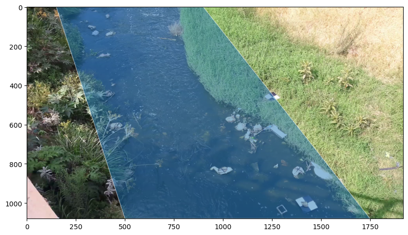
Extract one frame with stabilization window#
Below, let’s have a look how the stabilization window encompasses the water surface. By including this, any area outside of the water is assumed (in the real world) to be stable and not moving, and any movements found there can then be corrected.
[3]:
# some keyword arguments for fancy polygon plotting
patch_kwargs = {
    "alpha": 0.5,
    "zorder": 2,
    "edgecolor": "w",
    "label": "Area of interest",
}
f, ax = plt.subplots(1, 1, figsize=(10, 6))

frame = video.get_frame(0, method="rgb")
# plot frame on a notebook-style window
ax.imshow(frame)
# add the polygon to the axes
patch = patches.Polygon(
    stabilize,
    **patch_kwargs
)
p = ax.add_patch(patch)
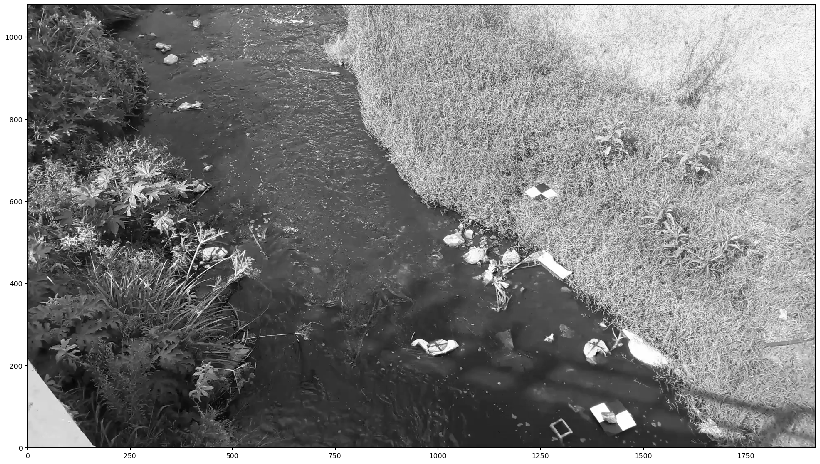
extracting gray scaled frames#
You can see the video holds information about the video itself (filename, fps, and so on) but also the camera configuration supplied to it. We can now extract the frames. Without any arguments, the frames are automatically grayscaled and all frames are extracted.
[4]:
da = video.get_frames()
da
[4]:
<xarray.DataArray 'frames' (time: 126, y: 1080, x: 1920)> Size: 261MB
dask.array<concatenate, shape=(126, 1080, 1920), dtype=uint8, chunksize=(20, 1080, 1920), chunktype=numpy.ndarray>
Coordinates:
  * time     (time) float64 1kB 0.0 0.03333 0.06667 0.1 ... 4.1 4.133 4.167
  * y        (y) int64 9kB 1079 1078 1077 1076 1075 1074 1073 ... 6 5 4 3 2 1 0
  * x        (x) int64 15kB 0 1 2 3 4 5 6 ... 1913 1914 1915 1916 1917 1918 1919
    xp       (y, x) int64 17MB 0 1 2 3 4 5 6 ... 1914 1915 1916 1917 1918 1919
    yp       (y, x) int64 17MB 1079 1079 1079 1079 1079 1079 ... 0 0 0 0 0 0
Attributes:
    camera_shape:   [1080, 1920]
    camera_config:  {\n    "height": 1080,\n    "width": 1920,\n    "crs": "P...
    h_a:            0.0
chunksize: 20The frames object is really a xarray.DataFrame object, with some additional functionalities under the method .frames. The beauty of our API is that it also uses lazy dask arrays to prevent very lengthy runs that then result in gibberish because of a small mistake along the way. We can see the shape and datatype of the end result, without actually computing everything, until we request a sample. Let’s have a look at only the first frame with the plotting functionalities. If you want to
use the default plot functionalities of xarray simply replace the line below by:
da[0].plot(cmap="gray")
[5]:
da[0].frames.plot(cmap="gray")
[5]:
<matplotlib.image.AxesImage at 0x7f31c04ab980>
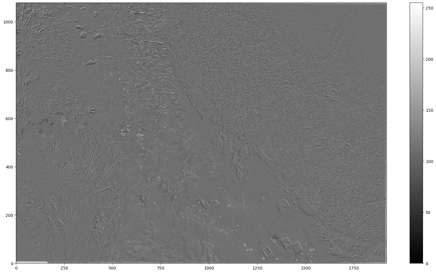
normalize to add contrast#
the .frames methods hold functionalities to improve the contrast of the image. A very good step is to remove the average of a larger set of frames from the frames itself, so that only strongly contrasting patterns from the background are left over. These are better traceable. We do this with the .normalize method. By default, 15 samples are used.
[6]:
# da_norm = da.frames.time_diff(abs=False, thres=0.)
# da_norm = da_norm.frames.minmax(min=0.)
da_norm = da.frames.normalize()
p = da_norm[0].frames.plot(cmap="gray")
plt.colorbar(p)
[6]:
<matplotlib.colorbar.Colorbar at 0x7f31b8c73d40>
A lot more contrast is visible now. We can now project the frames to an orthoprojected plane. The camera configuration, which is part of the Video object is used under the hood to do this. We use the new numpy-based projection method. The default is to use OpenCV methods, remove method="numpy" to try that.
[7]:
f = plt.figure(figsize=(16, 9))
da_norm_proj = da_norm.frames.project(method="numpy")
da_norm_proj[0].frames.plot(cmap="gray")
[7]:
<matplotlib.image.AxesImage at 0x7f31b8b16630>
<Figure size 1600x900 with 0 Axes>
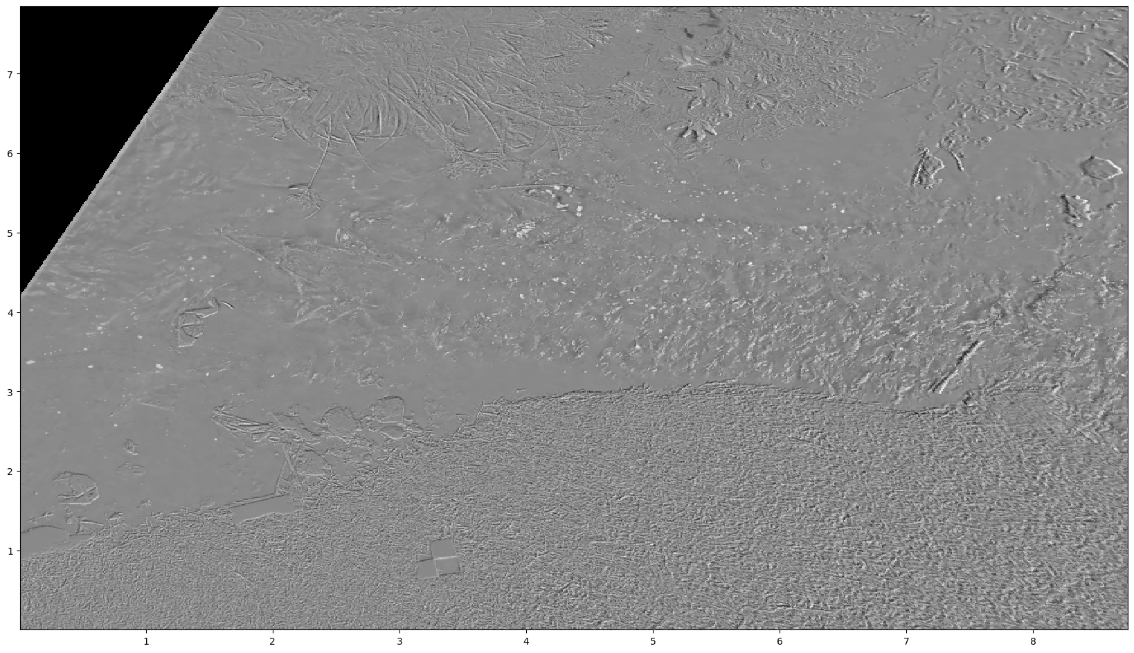
You can see that the frames now also have x and y coordinates. These are in fact geographically aware, because we measured control points in real world coordinates and added a coordinate reference system to the CameraConfig object (see notebook 01). The DataArray therefore also contains coordinate grids for lon and lat for longitudes and latitudes. Hence we can also go through this entire pipeline with an RGB image and plot this in the real world by adding mode="geographical"
to the plotting functionalities. The grid is rotated so that its orientation always can follow the stream (in the local projection shown above, left is upstream, right downstream). Plotting of an rgb frame geographically is done as follows:
[8]:
# extract frames again, but now with rgb
da_rgb = video.get_frames(method="rgb")
# project the rgb frames, same as before
da_rgb_proj = da_rgb.frames.project()
# plot the first frame in geographical mode
p = da_rgb_proj[0].frames.plot(mode="geographical")

# for fun, let's also add a satellite background from cartopy
import cartopy.io.img_tiles as cimgt
import cartopy.crs as ccrs
tiles = cimgt.GoogleTiles(style="satellite")
p.axes.add_image(tiles, 19)
# zoom out a little bit so that we can actually see a bit
p.axes.set_extent([
    da_rgb_proj.lon.min() - 0.0001,
    da_rgb_proj.lon.max() + 0.0001,
    da_rgb_proj.lat.min() - 0.0001,
    da_rgb_proj.lat.max() + 0.0001],
    crs=ccrs.PlateCarree()
)
Velocimetry estimates#
Now that we have real-world projected frames, with contrast enhanced, let’s do some velocimetry! For Particle Image Velocimetry, this is as simple as calling the .get_piv method on the frames. We then store the result in a nice NetCDF file. This file can be loaded back into memory with the xarray API without any additional fuss.
[9]:
piv = da_norm_proj.frames.get_piv()
piv.to_netcdf("ngwerere_piv.nc")
Computing PIV per chunk: 100%|██████████| 2/2 [00:12<00:00, 6.38s/it]
Beautiful additions to your art gallery#
Of course now we want to do some plotting and filtering, for that, please go to the next notebook