Camera configurations#
An essential element in doing optical velocity estimates is understanding how the Field Of View (FOV) of a camera relates to the real-world coordinates. This is needed so that a camera’s FOV can be “orthorectified”, meaning it can be transposed to real-world coordinates with equal pixel distances in meters. For this we need understanding of the lens characteristics, and understanding of where a pixel (2-dimensional with column and row coordinates, a.k.a. image coordinates) is located in the real world (3-dimensional, a.k.a. geographical coordinates). The camera configuration methods of pyorc are meant for this purpose.
Setting up a camera configuration#
The command-line interface supports setting up a camera configuration through a subcommand. To see the options
simply call the subcommand on a command prompt with --help as follows:
$ pyorc camera-config --help
Usage: pyorc camera-config [OPTIONS] OUTPUT

  CLI subcommand for camera configuration.

Options:
  -V, --videofile FILE        video file with required objective and
                              resolution and control points in view
                              [required]
  --crs TEXT                  Coordinate reference system to be used for
                              camera configuration
  -f, --frame-sample INTEGER  Frame number to use for camera configuration
                              background
  --src TEXT                  Source control points as list of [column, row]
                              pairs.
  --dst TEXT                  Destination control points as list of 2 or 4 [x,
                              y] pairs, or at least 6 [x, y, z]. If --crs_gcps
                              is provided, --dst is assumed to be in this CRS.
  --z_0 FLOAT                 Water level [m] +CRS (e.g. geoid or ellipsoid of
                              GPS)
  --h_ref FLOAT               Water level [m] +local datum (e.g. staff or
                              pressure gauge)
  --crs_gcps TEXT             Coordinate reference system in which destination
                              GCP points (--dst) are measured
  --resolution FLOAT          Target resolution [m] for ortho-projection.
  --focal_length FLOAT        Focal length [pix] of lens.
  --k1 FLOAT                  First lens radial distortion coefficient k1 [-].
                              See also https://docs.opencv.org/2.4/modules/cal
                              ib3d/doc/camera_calibration_and_3d_reconstructio
                              n.html
  --k2 FLOAT                  Second lens radial distortion coefficient k2
                              [-]. See also https://docs.opencv.org/2.4/module
                              s/calib3d/doc/camera_calibration_and_3d_reconstr
                              uction.html
  --window_size INTEGER       Target window size [px] for interrogation window
                              for Particle Image Velocimetry
  --shapefile FILE            Shapefile or other GDAL compatible vector file
                              containing dst GCP points [x, y] or [x, y, z] in
                              its geometry
  --lens_position TEXT        Lens position as [x, y, z]. If --crs_gcps is
                              provided, --lens_position is assumed to be in
                              this CRS.
  --corners TEXT              Video ojective corner points as list of 4
                              [column, row] points
  -s, --stabilize             Stabilize the videos using this camera
                              configuration (you can provide a stable area in
                              an interactive view).
  --rotation INTEGER          Provide a rotation of either 90, 180 or 170
                              degrees if needed to correctly rotate the video
  -v, --verbose               Increase verbosity.
  --help                      Show this message and exit.
To setup a camera configuration, you will at minimum need to provide the following:
A video, made with a specific camera, oriented to a fixed point of view, using known and fixed settings. With “fixed” we mean here that any additional video supplied to pyorc should be taken with the same settings and the same exact field of view.
Ground control points. These are combinations of real-world coordinates (possibly in a geographical coordinate reference system) and column, row coordinates in the frames of the video. By assigning where in the world a column, row coordinate is, and do this for several locations, the field of view of the camera can be projected into a real-world view.
4 corner points that approximately indicate the bounding box of your area of interest. These must be provided in the order upstream-left, downstream-left, downstream-right, upstream-right, where left is the left-bank as seen while looking in downstream direction. An exception is when you have a nadir drone video. In this case, it may be assumed that the entire view is relevant. In the Command-Line interface you can then skip providing corner points.
If you wish to use the video only from a selected frame (for instance if the first frames/seconds are bad quality, or moving) then you must also provide the frame number from which you would like to start the analysis and provide the camera configuration information. This is done with the
-for--frame-sampleoption. In the interactive views that will support you, this frame will be displayed. If you do not provide-fthen the first frame (index 0) will be displayed.
There are several ways to assign this information, further explained below.
In pyorc all camera configuration is collected into one single class called CameraConfig. It can be imported
from the main library and then be used to add information about the lens characteristics and the relation between
real-world and row-column coordinates. Once completed, the camera configuration can be added to a video to make it lens
and geographically aware. You can also add a camera configuration, stored in a JSON-formatted file to a video.
Once this is done, the video has added intelligence about the real-world, and you can orthorectify its frames.
Below a simple example is shown, where only the expected size of the objective in height and width is provided.
import pyorc
cam_config = pyorc.CameraConfig(height=1080, width=1920)
cam_config

{
    "height": 1080,
    "width": 1920,
    "resolution": 0.05,
    "window_size": 10,
    "dist_coeffs": [
        [
            0.0
        ],
        [
            0.0
        ],
        [
            0.0
        ],
        [
            0.0
        ]
    ],
    "camera_matrix": [
        [
            1920.0,
            0.0,
            960.0
        ],
        [
            0.0,
            1920.0,
            540.0
        ],
        [
            0.0,
            0.0,
            1.0
        ]
    ]
}
You can see that the inline representation of the CameraConfig object is basically a dictionary with pieces of
information in it. In this example we can already see a few components that are estimated from default values. These
can all be modified, or updated with several methods after the object has been established. The different parts we can
see here already are as follows:
heightandwidth: these are simply the height and width of the expected objective of a raw video. You must at minimum provide these to generate aCameraConfigobject.resolution: this is the resolution in meters, in which you will get your orthoprojected frames, once you have a completeCameraConfigincluding information on geographical coordinates and image coordinates, and a bounding box, that defines which area you are interested in for velocity estimation. As you can see, a default value of 0.05 is selected, which in many cases is suitable for velocimetry purposes.window_size: this is the amount of orthorectified pixels in which one may expect to find a pattern and also. the size of a window in which a velocity vector will be generated. A default is here set at 10. In smaller streams you may decide to reduce this number, but we highly recommend not to make it lower than 5, to ensure that there are enough pixels to distinguish patterns in. If patterns seem to be really small, then you may decide to reduce the resolution instead. pyorc automatically uses an overlap between windows of 50% to use as much information as possible over the area of interest. With the default settings this would mean you would get a velocity vector every 0.05 * 10 / 2 = 0.25 meters.dist_coeffs: this is a vector of at minimum 4 numbers defining respectively radial (max. 6) and tangential (2) distortion coefficients of the used camera lens. As you can see these default to zeros only, meaning we assume no significant distortion if you do not explicitly provide information for this.camera_matrix: the intrinsic matrix of the camera lens, allowing to transform a coordinate relative to the camera lens coordinate system (still in 3D) into an image coordinate (2D, i.e. a pixel coordinate). More on this can be found e.g. on this blog.
As you can see, the camera configuration does not yet have any real-world information and therefore is not sufficient to perform orthorectification. Below we describe how you can establish a full camera configuration.
Making the camera configuration geographically aware#
In case you are able to perform your field measurements with a RTK GNSS device, then your camera configuration
can be made entirely geographically aware. You can then export or visualize your results in a geographical map later
on, or use your results in GIS software such as QGIS. You do this simply by passing the keyword crs (or --crs
on command line) to the camera configuration and enter a projection. Several ways to pass a projection are possible such as:
EPSG codes (see EPSG.io)
proj4 strings
Well-Know-Text format strings (WKT)
Because pyorc intends to measure velocities in distance metrics, it is compulsory to select a locally valid meter projected coordinate reference system, and not for instance an ellipsoidal coordinate system such as the typical WGS84 latitude longitude CRS. For instance in the Netherlands you may use Rijksdriehoek (EPSG code 28992). In Zambia the UTM35S projection (EPSG code 32735) is appropriate, whilst in Tanzania, we may select the UTM37S projection (EPSG code 32737). IF you use a non-appropriate or non-local system, you may get either very wrong results, or get errors during the process. To find a locally relevant system, we strongly recommend to visit the EPSG site and search for your location. If you do not have RTK GNSS, then simply skip this step and ensure you make your own local coordinate system, with unit meter distances.
Once your camera configuration is geographically aware, we can pass all other geographical information we may need in any projection, as long as we notify the camera configuration which projection that is. For instance, if we measure our ground control points (GCPs, see later in this manual) with an RTK GNSS set, and store our results as WGS84 lat-lon points, then we do not have to go through the trouble of converting these points into the system we chose for our camera configuration. Instead we just pass the CRS of the WGS84 lat-lon (e.g. using the EPSG code 4326) while we add the GCPs to our configuration. We will see this later in this manual.
To provide a geographical coordinate reference system to your camera configuration,
you may simply add the option --crs to the earlier command. Below an example
is given where as local projection, the UTM37S projection is provided. This projection
has EPSG code 32737 and is for instance applicable over Tanzania. A projection is meant
to provide a mostly undistorted real distance map for a given area. Because the globe
is round, a suitable projection system must be chosen, that belongs to the area of
interest. Visit https://epsg.io/ to find a good projection system for your area of
interest.
$ pyorc camera-config --crs 32737 ........
The dots represent additional required to make a full camera configuration.
If you provide a list of real-world ground control points in the command-line interface, and you supply --crs,
then the real-world coordinates will be assumed to have the CRS WGS84 lat-lon. If this is not the case, then
you MUST provide the CRS of the real-world coordinates with the option --gcps_crs. This will then be used to
transform the coordinates provided to the CRS provided with --crs. If you do not provide --gcps_crs.
Below, we show what the configuration would look like if we would add the Rijksdriehoek projection to our camera configuration. You can see that the code is converted into a Well-Known-Text format, so that it can also easily be stored in a generic text (json) format.
import pyorc
cam_config = pyorc.CameraConfig(height=1080, width=1920, crs=32631)
cam_config

{
    "height": 1080,
    "width": 1920,
    "crs": "PROJCRS[\"WGS 84 / UTM zone 31N\",BASEGEOGCRS[\"WGS 84\",ENSEMBLE[\"World Geodetic System 1984 ensemble\",MEMBER[\"World Geodetic System 1984 (Transit)\"],MEMBER[\"World Geodetic System 1984 (G730)\"],MEMBER[\"World Geodetic System 1984 (G873)\"],MEMBER[\"World Geodetic System 1984 (G1150)\"],MEMBER[\"World Geodetic System 1984 (G1674)\"],MEMBER[\"World Geodetic System 1984 (G1762)\"],MEMBER[\"World Geodetic System 1984 (G2139)\"],ELLIPSOID[\"WGS 84\",6378137,298.257223563,LENGTHUNIT[\"metre\",1]],ENSEMBLEACCURACY[2.0]],PRIMEM[\"Greenwich\",0,ANGLEUNIT[\"degree\",0.0174532925199433]],ID[\"EPSG\",4326]],CONVERSION[\"UTM zone 31N\",METHOD[\"Transverse Mercator\",ID[\"EPSG\",9807]],PARAMETER[\"Latitude of natural origin\",0,ANGLEUNIT[\"degree\",0.0174532925199433],ID[\"EPSG\",8801]],PARAMETER[\"Longitude of natural origin\",3,ANGLEUNIT[\"degree\",0.0174532925199433],ID[\"EPSG\",8802]],PARAMETER[\"Scale factor at natural origin\",0.9996,SCALEUNIT[\"unity\",1],ID[\"EPSG\",8805]],PARAMETER[\"False easting\",500000,LENGTHUNIT[\"metre\",1],ID[\"EPSG\",8806]],PARAMETER[\"False northing\",0,LENGTHUNIT[\"metre\",1],ID[\"EPSG\",8807]]],CS[Cartesian,2],AXIS[\"(E)\",east,ORDER[1],LENGTHUNIT[\"metre\",1]],AXIS[\"(N)\",north,ORDER[2],LENGTHUNIT[\"metre\",1]],USAGE[SCOPE[\"Engineering survey, topographic mapping.\"],AREA[\"Between 0\u00b0E and 6\u00b0E, northern hemisphere between equator and 84\u00b0N, onshore and offshore. Algeria. Andorra. Belgium. Benin. Burkina Faso. Denmark - North Sea. France. Germany - North Sea. Ghana. Luxembourg. Mali. Netherlands. Niger. Nigeria. Norway. Spain. Togo. United Kingdom (UK) - North Sea.\"],BBOX[0,0,84,6]],ID[\"EPSG\",32631]]",
    "resolution": 0.05,
    "window_size": 10,
    "dist_coeffs": [
        [
            0.0
        ],
        [
            0.0
        ],
        [
            0.0
        ],
        [
            0.0
        ]
    ],
    "camera_matrix": [
        [
            1920.0,
            0.0,
            960.0
        ],
        [
            0.0,
            1920.0,
            540.0
        ],
        [
            0.0,
            0.0,
            1.0
        ]
    ]
}
Note
A smart phone also has a GNSS chipset, however, this is by far not accurate enough to provide the measurements needed for pyorc. We recommend using a (ideal!) RTK GNSS device with a base station setup close enough to warrant accurate results, or otherwise a total station or spirit level. Highly affordable GNSS kits with base and rover stations are available through e.g. ardusimple.
Camera intrinsic matrix and distortion coefficients#
An essential component to relate the FOV to the real world is the camera’s intrinsic parameters, i.e. parameters that define the dimensions and characteristics of the used camera lens and its possible distortion. As an example, a smartphone camera has a very flat lens, with a short focal distance. This often results in the fact that objects or people at the edges of the field of view seem stretched, while the middle is quite reliable as is. With a simple transformation, such distortions can be corrected. Fish eye lenses, which are very popular in trail cameras, IP cameras and extreme sport cameras, are constructed to increase the field of view at the expense of so-called radial distortions. With such lenses, straight lines may become distorted into bend lines in your objective. Imagine that this happens with a video you wish to use for velocimetry, then your geographical referencing can easily be very wrong (even in the order of meters with wide enough streams) if you do not properly account for these. If for example your real-world coordinates are measured somewhere in the middle of the FOV, then velocities at the edges are likely to be overestimated.
Note
In pyorc the focal distance is automatically optimized based on your real-world coordinates, provided as ground control points. This is done already if you provide 4 control points in one vertical plane (e.g. at the water level). In case you provide 6 or more ground control points with varying vertical levels, then pyorc will also attempt to optimize the radial distortion. Therefore we strongly recommend that you measure 6 or more control points in case you use a lens with significant radial distortion.
You can also provide a camera intrinsic matrix and distortion coefficients in the CLI or API if you have these, or optimize the intrinsic matrix and distortion coefficients using a checkerboard pattern. More on this is described below.
Preparing a video for camera calibration#
We have a method available to manually establish an intrinsic matrix and distortion coefficients. It reads in a video in which a user shows a chessboard pattern and holds it in front of the camera in many different poses and at as many different locations in the field of view as possible. It then strips frames in a staggered manner starting with the first and last frame, and then the middle frame, and then the two frames in between the first, last and middle, and so on, until a satisfactory number of frames have been found in which the chessboard pattern was found. The intrinsic matrix and distortion coefficients are then calculated based on the results, and added to the camera configuration.
Note
Making a video of a chessboard pattern and calibrating on it is only useful if you do it the right way. Take care of the following guidelines:
ensure that the printed chessboard is carefully fixed or glued to a hard object, like a strong straight piece of cardboard or a piece of wood. Otherwise, the pattern may look wobbly and cause incorrect calibration
a larger chessboard pattern (e.g. A0 printed) shown at a larger distance may give better results because the focal length is more similar to field conditions. An A4 printed pattern is too small. Using pyorc’s built-in calibration is then more trustworthy.
make sure that while navigating you cover all degrees of freedom. This means you should move the checkerboard from top to bottom and left to right; in all positions, rotate the board around its horizontal and vertical middle line; and rotate it clockwise.
make sure you record the video in exactly the same resolution and zoom level as you intend to use during the taking of the videos in the field.
If the calibration process is not carefully followed it may do more harm than good!!! Therefore, if you are unsure then we strongly recommend simply relying on the built-in automated calibration.
An example of extracts from a calibration video with found corner points is shown below (with A4 printed chessboard so not reliable for a field deployment, this is only an example). It gives an impression of how you can move the chessboard pattern around. As said above, it is better to print a (much!) larger chessboard and show that to the camera at a larger distance.
Lens calibration method#
Note
At the moment, manual lens calibration is only available at API level. If you require a command-line option for lens calibration, then please contact us at info@rainbowsensing.com. If you have the focal length, and k1 and k2 radial distortion parameters available, then you can enter these in the command line interface using the –focal_length, –k1, –k2 parameters. The units of the focal length should be in pixels. For focal length, and distortion parameters, we use the OpenCV methods, so please ensure you use the same as input here. For more information please read: the OpenCV instructions
Once you have your video, the camera calibration is very simple. After creating your camera configuration you can supply the video in the following manner:
calib_video = "calib_video.mp4"
cam_config.set_lens_calibration(calib_video)
When you execute this code, the video will be scanned for suitable images, and will select frames that are relatively far apart from each other. When a suitable image with patterns is found, the algorithm will show the image and the found chessboard pattern. There are several options you may supply to the algorithm to influence the amount of internal corner points of the chessboard (default is 9x6), the maximum frames number that should be used for calibration, filtering of poorly performing images, switch plotting and writing plots to files (for later checking of the results) on or off.
Note
the camera calibration is still experimental. If you have comments or issues kindly let us know by making a github issue.
Ground control points#
Besides the characterization of the lens used for taking the video, we must also characterise the camera to real-world coordinate system. In other words: we must know where a row and column in our camera perspective may lie in the real world. Naturally, this is a poorly defined problem as your camera’s perspective can only be 2D, whilst the real world has 3 dimensions. However, our problem is such that we can always fix one dimension, i.e. the elevation. If we already know and fix the level of the water (z-coordinate), then we can interpret the remaining x-, and y-coordinates if we give the camera calibration enough information to interpret the perspective. We do this by providing so-called ground control points, that are visible in the FOV, and of which we know the real-world coordinates.
ground control point information and abbreviations#
Within pyorc, both the command-line inteface and API, the different components of your ground control points are represented by abbreviated variables. These have the following meaning:
srccontains [column, row] locations of the control points in the FOV.dst: contains [x, y] locations (in case you use 4 control points on one vertical plane) or [x, y, z] locations ( in case you use 6 control points with arbitrary elevation).z_0: water level measured in the vertical reference of your measuring device (e.g. RTK GNSS)h_ref: water level as measured by a local measurement device such as a staff gaugecrs: the CRS in which the control points are measured. This can be different from the CRS of the camera configuration itself in which case the control points are automatically transformed to the CRS of the camera configuration. If left empty, then it is assumed the CRS of the measured points and the camera configuration is the same.
Measuring the GCP information#
Below we describe how the information needed should be measured in the field during a dedicated survey. This is typically done every time when you do an incidental observation, or once during the installation of a fixed camera. If you leave the camera in place, you can remove recognizeable control points after the survey, as long as you have one video with the control points visible, which you can use to setup the camera configuration.
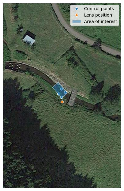
Example of survey situations#
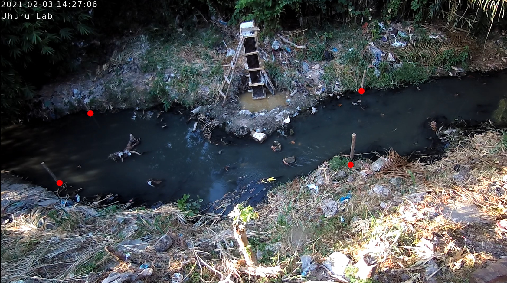
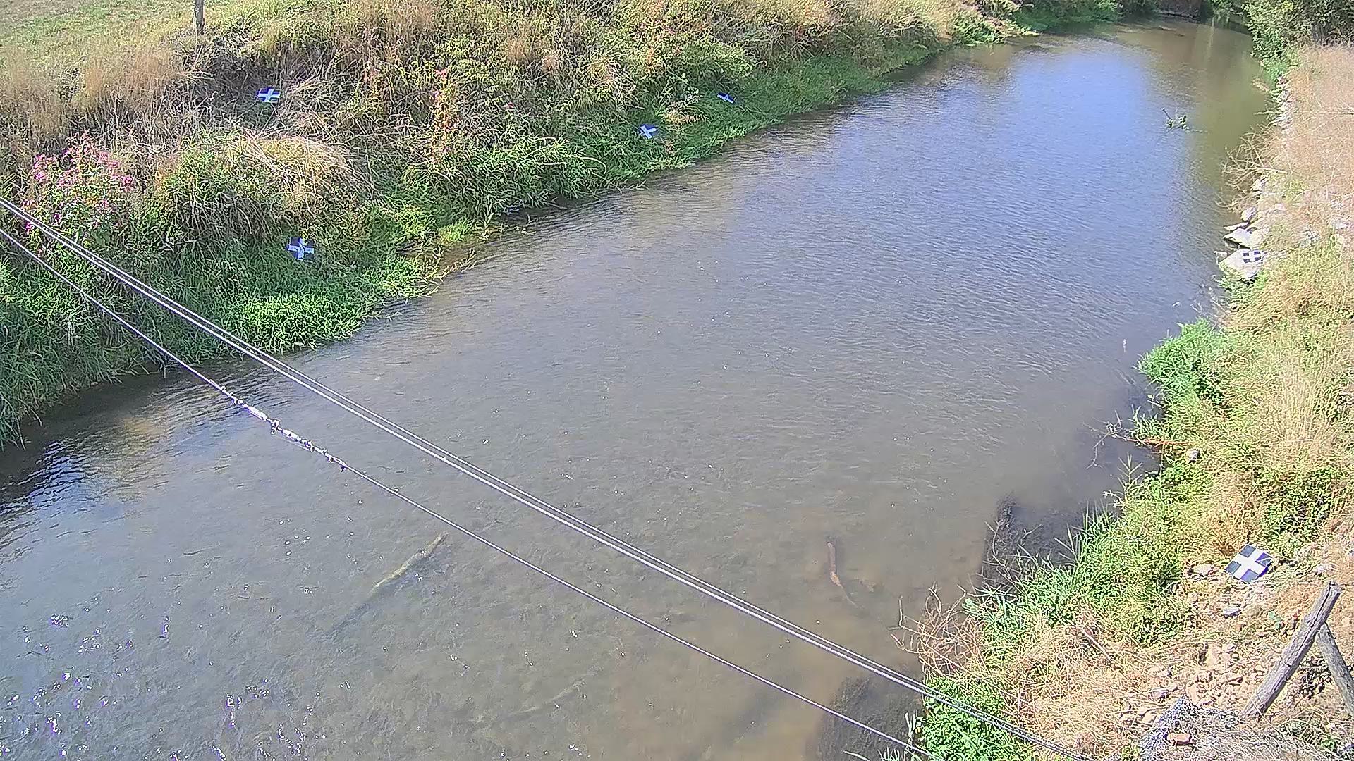
You will notice in the next sections that you can typically measure either 4 control points at one vertical plane (e.g. the water surface) or 6 or more points at random elevations. You prepare this situation by spreading easy to recognize markers over your Field of View. In the figure below you see two examples, one where 4 sticks were placed in the water and the interface of the sticks with the water (red dots) is measured. And one where 6 black-and-white markers are spread over the field of view.
4 GCPt at water surface - Chuo Kikuu River, Dar es Salaam, Tanzania |
|
6 (+) GCPs spread over banks and FOV - Geul River, Limburg, The Netherlands |
|
The schematic below shows in a planar view what the situation looks like. It is important that the control points are nicely spread over the Field of View, and this is actually more important than an equal spread of points of left and right bank. In the schematic we show this by having only 2 control points at the bank close to the camera, and 4 at the opposite side. If you have your camera on a bridge in the middle of the bridge deck, then having 3 (or more) points left as well as right makes the most sense. The better the spread is, the more accurate the perspective will be resolved.

Planar schematic view of site survey situation.#
Ensuring that the vertical plane is fully understood is also important.
The z_0 and h_ref optional keys are meant to allow a user to provide multiple videos with different water
levels. If you intend to do this, you may install a water level measuring device on-site such as a staff gauge or
pressure gauge, that has its own vertical zero-level reference. Therefore, to use this option the following should be
measured and entered:
measure the water level during the survey with your local device (e.g. staff gauge) and insert this in
h_refalso measure the water level with your survey device such as total station or RTK GPS, i.e. using the exact same vertical reference as your control points. This has its own vertical zero level. This level must be inserted in
z_0. Any other surveyed properties such as the lens position and the river cross section must also be measured with the same horizontal and vertical coordinate system asz_0and the ground control points.
The overview of these measurement requirements is also provided in the schematic below.

Cross-section schematic view of site survey situation.#
Entering control points in the camera configuration#
There are several approaches to provide ground control point information to the camera configuration through the command-line interface:
supply information with optional arguments as strings
supply information embedded in vector GIS files such as shapefiles
supply information interactively through (dependent on which information) a user-prompt or a visual interactive view.
For the first option, JSON-formatted strings are used. JSON is a standard format to provide information in string format
such as simple text, floating point numbers, integer numbers, but also more complex dictionaries, or lists. In our case
we only need floating point numbers to provide z_0 and h_ref, list of lists for src and dst and an
integer or string for --crs_gcps (i.e. the crs in which the destination locations of ground control points are
measured). Remember that --crs_gcps can be supplied through e.g. an EPSG code, which is an integer number, but also
in a “Well-known Text” (wkt) form, which is a string.
Note
In JSON format, a list can be supplied using comma separated numbers, encapsulated by square brackets “[” and “]”.
For our example video, supplying the gcps in a full command-line option manner would be done as follows:
$ pyorc camera-config --crs_gcps 32735 --src "[[1421, 1001], [1251, 460], [421, 432], [470, 607]]" --dst "[[642735.8076, 8304292.1190], [642737.5823, 8304295.593], [642732.7864, 8304298.4250], [642732.6705, 8304296.8580]]" --z_0 1182.2 --h_ref 0.0 ......
At the end of this command, after the ..... more inputs such as the video with control points, the CRS of the camera
configuration, and the output filename must be presented. With this input, no further interaction with the user to
complete the control points is required.
In many cases though, the information under -dst may be cumbersome to insert. Hence a more convenient option is to
leave out -dst and replace it for --shapefile and provide a path to a shapefile or other vector formatted
GIS file containing your real-world control points. pyorc assumes that the shapefile contains exactly those points you
wish to use, no more and no less, that all information is in the geometries (i.e. x, y and if +6-points are used, also z) and
that the file contains a CRS that allows for automated reprojection to the CRS of the camera configuration (i.e.
supplied with --crs). The geometries MUST be of the type POINT only! pyorc will attempt to indicate any
problems with shapefiles that contain wrong or incomplete information so that you can resolve that if needed.
Note
If you use a RTK GNSS, a typical output is a shapefile containing points, a CRS and geometries with x, y and z coordinates. If your output file contains more points than your control points, then first edit the file in a GIS program such as QGIS and delete any points that do not belong to ground control points.
Similarly, the information contained in --src may also be very cumbersome to collect. In fact, you need to open up
a frame in a photo editor and note down rows and columns to do so. Therefore a much more and highly recommended
approach is to simply leave out -src entirely. You will then be asked if you want to interactively select these
points. Simply select Y and use our convenient point and click approach to select the control points. To make sure you
click them in the right order, you can click on the Map button to display a map overview of the situation. Here, your
--dst points (or points collected from the shapefile) will be displayed in a map view, with numbers indicating
which point should be selected first, which second and so on. You can go back to the camera view with the camera
button. Then you simply click on the first, second, third, … and so on control point to collect all control points.
Did you make an accidental click on a random point? No problem: just right-click and the last point you clicked
will be removed. Right-click again and the point before that is removed so that you can click again.
Once all point are clicked, pyorc will optimize both the perspective and the camera’s lens characteristics simultaneously, and display the points you clicked, but then projected using the camera matrix, distortion coefficients and the estimated perspective pose of the camera. You will see the result as red “+” signs on the screen and an average error in meters displayed on the top of the frame. If the average error is larger than 0.1 meter you will get a warning. Large errors are likely due to poorly measured control points, or because you clicked the points in the wrong order.
Once the optimization is performed, the Done button will become clickable. Click Done to close the view and store the points in the camera configuration. If you made a mistake and want to rectify poorly clicked points, simply right click as many times as needed to remove points, and add them again with left clicks. The optimization will be repeated again once you have reached the total amount of control points. The view after the optimization is shown in the example below.
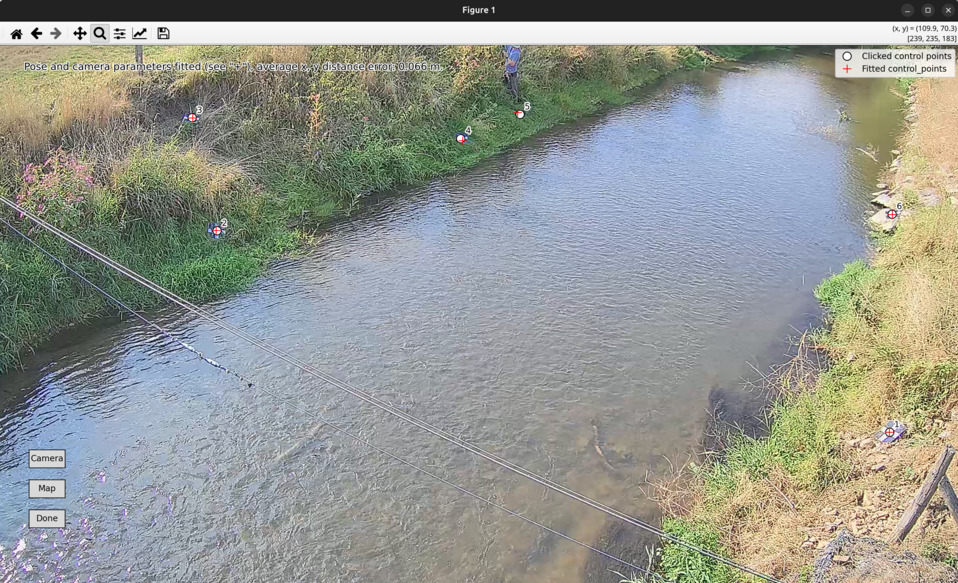
Note
Especially with large objectives and high resolution footage (e.g. 4K), it may be hard to accurately click or even see the control points. In this case, we highly recommend to use the zoom and pan functionality on the top bar of the interactive view. The Home button will bring you back to the original view.
The ground control points are a simple python dictionary that should follow a certain schema. The schema looks as follows:
{
    "src": [
        [int, int],
        [int, int],
        ...,
    ],
    "dst": [
        [float, float, Optional(float)],
        [float, float, Optional(float)],
        ...,
    ],
    "z_0": Optional(float),
    "h_ref": Optional(float),
    "crs": Optional(int, str)

}
The coordinates in the src field are simply the pixel coordinates in your video, where the GCPS are located.
You can look these up by plotting the first frame with plt.imshow or storing
the first frame to a file and open that in your favorite photo editor and count the pixels there.
dst contains the real-world coordinates, that belong to the same points, indicated in src.
dst must therefore contain either 4 x, y (if the left situation is chosen) or 6 x, y, z coordinates (if the right
situation is chosen.
In both cases you provide the points as a list of lists.
z_0 must be provided if 6 randomly placed points are used. If you intend to provide multiple videos with a locally
measured water level, then also provide h_ref as explained above. In case you have used 4 x, y points at the water surface, then also provide z_0. With this information
the perspective of the water surface is reinterpreted with each video, provided that a water level (as measured with the
installed device) is provided by the user with each new video.
Note
For drone users that only make nadir aimed videos, we are considering to also make an option with only 2 GCPs
possible. If you are interested in this, kindly make an issue in GitHub. For the moment we suggest to use the 4
control point option and leave z_0 and h_ref empty.
Finally a coordinate reference system (CRS) may be provided, that indicates in which CRS the survey was done if this
is available. This is only useful if you also have provided a CRS when creating the camera configuration. If you
for instance measure your control points in WGS84 lat-lon (EPSG code 4326) then pass crs=4326 and your coordinates
will be automatically transformed to the local CRS used for your camera configuration.
A full example that supplies GCPs to the existing camera configuration in variable cam_config is shown below:
src = [
    [1335, 1016],
    [270, 659],
    [607, 214],
    [1257, 268]
]  # source coordinates on the frames of the movie
dst = [
    [6.0478836167, 49.8830484917],
    [6.047858455, 49.8830683367],
    [6.0478831833, 49.8830964883],
    [6.0479187017, 49.8830770317]
]  # destination locations in long/lat locations, as measured with RTK GNSS.
z_0 = 306.595  # measured water level in the projection of the GPS device
crs = 4326  # coordinate reference system of the GPS device, EPSG code 4326 is WGS84 longitude/latitude.

cam_config.set_gcps(src=src, dst=dst, z_0=z_0, crs=crs)
If you have not supplied camera_matrix and dist_coeffs to the camera configuration, then these can be optimized
using the provided GCPs after these have been set using the following without any arguments.
cam_config.set_intrinsic()
Setting the lens position#
If you also provide a lens position, then this position will be used along-side the ground control points to better optimize the pose estimation and to better estimate the focal length. Similar to the control points, we advise to measure the location as accurately as possible, and naturally in exactly the same horizontal and vertical datum as the control points.
The position of the lens can be supplied with a simple list of [x, y, z] coordinate, provided within
quotes (“). It will be assumed that these coordinates share the same CRS as the ground control points. Hence if
you provide --crs_gcps or provide a shapefile with --shapefile that has a CRS embedded, then this CRS
will also be applied on the lens position. An example of how to supply the lens position with a pseudo-command
is provided below.
pyorc camera-config ... --lens_position "[642732.6705, 8304289.010, 1188.5]" ... OUTPUT.json
The lens position can be provided using a simple method set_lens_position. You only
need to provide x, y, z and the CRS (if this is different from the CRS of the camera configuration itself.
A full example supplying the lens position to the existing cam_config is shown below:
# cam_config object is already defined in earlier code blocks
lens_position = [6.0478872, 49.8830221, 309.8]  # lon, lat, elevation position of the camera
cam_config.set_lens_position(*lens_position, crs=4326)
Setting rotation#
If you are setting up a camera configuration on the CLI with a portrait video set up you may have to manually ensure
the video is rotated to portrait scale. With a smartphone video, this is usually detected automatically. With a
raspberry pi or IP camera this can usually not be detected. In this case, ensure that you manually provide the
--rotation flag with a valid value (90, 180 or 270 degrees). Also use the same angle when you perform velocimetry
on the same or other videos with the same view. See video rotation for more information.
Setting the area of interest#
pyorc is organized such that it processes a planar rectangular shaped area as shown in the example below over the Wark River in Luxembourg. The results of reprojection and velocity estimation will all fit in this area of interest in the form of raster maps. pyorc is also very flexible in the rotation of the grid. River sections almost never follow an ideal north-south or east-west direction, and therefore it is much more practical to allow for a rotated grid. This sounds complicated, but the great thing about pyorc is that you only have to supply 4 points in the camera Field of View and then pyorc will interpret for you where these 4 points lie in geographical space and which rectangular bounding box fits best around these points. In case there is a very clear dominant flow direction then we recommend to supply the corners points in a very specific order namely (see from the perspective looking in downstream direction):
upstream left-bank
downstream left-bank
downstream right-bank
upstream right-bank
Masking steps in pyorc where unreliable velocities are masked out can then also remove velocities that are in an unexpected direction more easily, and without tuning of masking parameters.
In the command-line interface there are three options to establish a bounding box to the camera configuration:
use the option
--cornersand supply a JSON-formatted list of 4 column, row pairs, similar to the approach used for supplying--src.use an interactive point-and-click view to click the points into your camera objective.
skip providing corners, and then pyorc will assume that the entire view is relevant. This is strictly only possible with nadir drone videos as in these cases, it may be assumed that no horizon is visible, and the area shown is limited. In the CLI this is detected by the amount of control points provided. If you have only provided two points, the assumption is that the video is nadir.
The --corners options works in exactly the same way as --src. pyorc uses the 4 corners to draw a geographical
best-fitting rectangular box automatically and add this to the camera configuration.
As said before, choosing these corner points may be something you wish to try out a few times to get it right.
Moreover, selecting them would also require a photo editor, and cumbersome noting down of coordinates and this can also
easily be prone to errors where you accidentally swap row or column, or accidentally supply data in the wrong order.
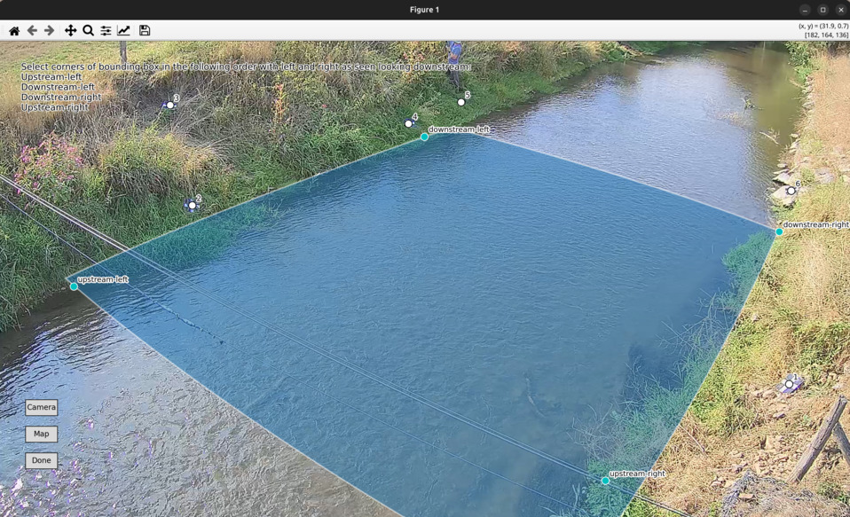
Similar to the --src case, you can also simply leave out --corners and then pyorc will ask if you wish to
interactively supply the corner points. Simply choose Y for yes, and you will again get an interactive view.
This view will show the earlier chosen --src points in the Camera view, and (if you click on Map) the -dst
points in the Map view. Once you start selecting corners points in the Camera view, the view will show you which
of the 4 points you have selected (e.g. the first point would read as “upstream left-bank”. COntinue until you have
clicked 4 points, and then you will see the allocated bounding box around the 4 points. If you then click on Map
you will see the same bounding box in geographical space. If you wish to improve your corner point selection, then
simply use right-click to remove points and select new locations for them to change the bounding box. Once you are
satisfied, click on Done and the bounding box will be stored in the camera configuration.
Below an example of the bounding box as it appears in the interactive interface is shown.
The area of interest can theoretically be provided directly, simply by providing
a shapely.geometry.Polygon with 5 bounding points as follows (pseudo-code):
cam_config.bbox = Polygon(...)
However, this is quite risky, as you are then responsible for ensuring that the area of interest is rectangular, has exactly 4 corners and fits in the FOV. Currently, there are no checks and balances in place, to either inform the user about wrongfully supplied Polyons, or Polygons that are entirely outside of the FOV.
Therefore, a much more intuitive approach is to use set_bbox_from_corners. You simply supply 4 approximate
corner points of the area of interest within the camera FOV. pyorc will then find the best planar bounding box
around these roughly chosen corner points and return this for you. A few things to bear in mind while choosing these:
Ensure you provide the corner points in the right order. So no diagonal order, but always along the expected Polygon bounds.
If you intend to process multiple videos with the same camera configuration, ensure you choose the points wide enough so that with higher water levels, they will likely still give a good fit around the water body of interest.
Important: if water follows a clear dominant flow direction (e.g. in a straight relatively uniform section) then you may use the angular filter later on, to remove spurious velocities that are not in the flow direction. In order to make the area of interest flow direction aware, ensure to provide the points in the following order:
upstream left-bank
downstream left-bank
downstream right-bank
upstream right-bank
where left and right banks are defined as if you are looking in downstream direction.
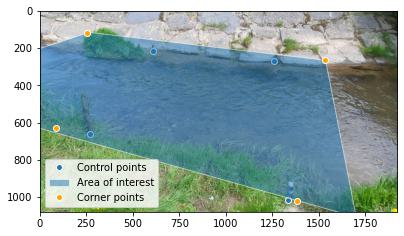
Below we show how the corners are provided to the existing cam_config.
corners = [
    [255, 118],
    [1536, 265],
    [1381, 1019],
    [88, 628]
]
cam_config.set_bbox_from_corners(corners)
This yields the bounding box shown in the figure above, which is the same as the one shown in the perspective below. You can see that the rectangular area is chosen such that the chosen corner points at least fit in the bounding box, and the orientation is chosen such that it follows the middle line between the chosen points as closely as possible.
An alternative approach is to use set_bbox_from_width_length. This works much better in case where a strong oblique
angle is used. You provide three points. The first two define the left-to-right width, and the last the length of the
bounding box in up- and downstream direction. This method makes it a lot easier to ensure that the chosen bounding box
is aligned with the flow direction. The approach to calling is the same as the previous, except you only supply 3
points.
points = [
    [255, 118],
    [1536, 265],
    [1381, 1019],
]
cam_config.set_bbox_from_width_length(points)
Stabilization#
You can decide whether videos must be stabilized. pyorc needs to be able to find so-called “rigid points” to do this. Rigid points are points that do not move during the video. pyorc can automatically detect easy stable points to track and then follow how these move from frame to frame. As the points should not move, pyorc will then transform each frame so that the resulting movements are minimized. To ensure the transformation are really rigid, such regid points must be found on all edges of the video. Hence it is important that when you take an unstable video, that there is enough visibility of surrounding banks, or infrastructure or other stable elements around the video to perform the stabilization. If such objects are only found in e.g. one half or (worse) one quadrant of the video, then the stabilization may give very strange results in the areas where no rigid points are found. Therefore, only use this if you know quite certainly that stable points will be found in many regions around the water.
For stabilization, pyorc requires a polygon that defines the area where no rigid points are expected. This is essentially the moving water and possibly also strongly moving vegetation if this is present in the frame. So select the polygon such that it encompasses both water and other strongly moving elements as much as possible.
On the command line, simply provide --stabilize or -s as additional argument and you will be provided
with a interactive point and click view on your selected frame. You may click as many points as you wih to
create a polygon that encompasses moving things. To ensure that you include all edges, you can also pan
the frame so that areas outside of the frame become visible. Select the 4th button from the left (two crossed
double-arrows) to select panning. Click on the most left (Home) button to return to the original view.
For stabilization, provide stabilize as additional argument to CameraConfig and provide as value
a list of lists of coordinates in [column, row] format, similar to gcps["src"].
Result of a camera configuration#
Once you have all your settings and details complete, the camera configuration can be stored, plotted and later used for processing videos into velocimetry.
When all required parameters are provided, the resulting camera configuration will be stored in a file
set as <OUTPUT> on the command line. If you have our code base and the examples folder, then you can for
instance try the following to get a camera configuration without any interactive user inputs required:
$ cd examples/ngwerere
$ pyorc camera-config -V ngwerere_20191103.mp4 --crs 32735 --z_0 1182.2 --h_ref 0.0 --lens_position "[642732.6705, 8304289.010, 1188.5]" --resolution 0.03 --window_size 15 --shapefile ngwerere_gcps.geojson --src "[[1421, 1001], [1251, 460], [421, 432], [470, 607]]" -vvv ngwerere_cam_config.json
This will use the video file ngwerere_20191103.mp4, make a camera configuration in the CRS with EPSG number
32735 (UTM Zone 35 South), with measured water level at 1182.2, and reference water level at 0.0 meter (i.e.
we only treat one video). The lens position, set as coordinates in UTM35S is set as an [x, y, z] coordinate,
resolution used for reprojection is set at 0.03 meter, with a window size for cross-correlation set at 15 pixels.
The destination control points are provided in a file ngwerere_gcps.geojson and the source coordinates
are provided as a list with [column, row] coordinates in the frame object. Finally, corner points to set the
bounding box are provided as a list of [column, row] coordinates as well. The configuration is stored in
ngwerere_cam_config.json. If you leave out the --src and --corners components, you will be able to
select these interactively as shown before. You can also add --stabilize to also provide a region for
stabilization as described before. Also the --h_ref and --z_0 values can be supplied
interactively on the command line.
The command-line interface will also automatically store visualizations of the resulting camera configuration
in both planar view (with a satellite background if a CRS has been used) and in the camera perspective. The file
names for this have the same name as <OUTPUT> but with the suffixes _geo.jpg for the planar view and
_cam.jpg for the camera FOV perspective.
After the configuration is stored, the CLI will ask if you want to receive a GeoTIFF of the projected frame. If you select “Yes”, this will be provided side-by-side with the camera configuration file.
Storing a camera configuration within the API is as simple as calling to_file. Camera configurations can
also be loaded back in memory using pyorc.load_camera_config.
# cam_config was generated before from our examples/ngwerere folder
import pyorc
cam_config.to_file("ngwerere_cam_config.json")
# load the configuration back in memory
cam_config2 = pyorc.load_camera_config("ngwerere_cam_config.json")
When a full camera configuration is available, you can access and inspect several properties and access a few other methods that may be useful if you wish to program around the API. We refer to the API documentation.
We highly recommend to first inspect your camera configuration graphically, before doing any further work with it.
Examples have already been shown throughout this manual, but you can also plot your own camera configurations, either
in planar view, or in the original camera FOV. For this the plot method has been developed. This method can
always be applied on an existing matplotlib axes object, by supplying the ax keyword and referring the the axes
object you wish to use.
Planar plotting is done by default. The most simple approach is:
cam_config.plot()
This will yield just the camera configuration information, and can always be used, whether you have a geographically
aware camera configuration (CRS provided) or not. If the camera configuration is geographically aware, then you
can also add a satellite or other open map as a background. pyorc uses the cartopy package to do this. You can
control this with the tiles keyword to define a tiles layer (see this page)
Additional keywords you may want to pass to the tiles set can be defined in the keyword tiles_kwargs. Finally, the
zoom level applied can be given in the keyword zoom_level. By default, a very high zoom level (18) is chosen,
because mostly, areas of interest cover only a small geographical region. The geographical view shown above can be
displayed as follows:
cam_config.plot(tiles="GoogleTiles", tiles_kwargs=dict(style="satellite"))
To plot in the camera FOV, simply set camera=True.
cam_config.plot(camera=True)
This may look a little awkward, because plotting in matplotlib is defaulting to having the 0, 0 point in the bottom left while your camera images have it at the top-left. Furthermore, you cannot really interpret what the FOV looks like. Hence it makes more sense to utilize one frame from an actual video to enhance the plotting. Here we use the video on which the camera configuration is based, extract one frame, and plot it within one axes.
fn = r"20220507_122801.mp4"
video = pyorc.Video(fn, camera_config=cam_config, start_frame=0, end_frame=1)

# get the first frame as a simple numpy array
frame = video.get_frame(0, method="rgb")
# combine everything in axes object "ax"
ax = plt.axes()
ax.imshow(frame)
cam_config.plot(ax=ax, camera=True)